LEARN TO explore

Accessing the AURIN API via RStudio

This tutorial is also available on the following GitHub repository: https://github.com/AURIN-OFFICE/training/tree/main/Explore/R

The goal of this tutorial is to demonstrate how to use RStudio to connect to the AURIN API and download data. This is designed with no prerequisite of experience using R.

The AURIN API is an interface that allows you to use programming scripts to access and interact with the AURIN Data Catalogue. Users can download specific datasets using R scripts to make retrieval requests to the API.

The API is based on Open Geospatial Consortium Web Feature Service (WFS) Interface Standards.

Before attempting the steps in this tutorial, please ensure you have generated your unique API Credentials (username and password) using the Access Dashboard. If you need guidance on creating your credentials, please refer to the tutorial here.

Please note the API access password will expire in 90 days for security reasons. You can always get a new password by visiting the API Access page.

Tutorial Goals

In this tutorial, our goal is to use RStudio to connect to the API and download a dataset. The following topics will be covered:

choosing between different R coding environments;
an introduction to R packages and libraries and how to install them; and
interacting with the API using the R coding environment.

1. Choose Between Different R Environments

R is a free and open-source programming language and environment for statistical computing and graphics. R can be a very powerful tool for data analysts from all disciplines. The geographic information system (GIS) capabilities of R have developed significantly over the last decade.

If you have no prior experience with R, a cloud environment such as posit Cloud which has R and its prerequisites already installed, can be a good starting point. If you wish to use your personal computer, we recommend using R version 4.3.2 or later. The image below lists the benefits and limitations of each option.

a) Cloud Environment

posit Cloud (formerly RStudio Cloud) is a cloud service in which to use RStudio and is accessible here.

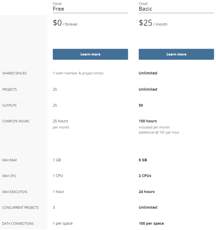
As the screenshot above shows, there are limitations on the free-of-charge tier of RStudio in posit Cloud. Specifically, the limitation of 1GB of RAM will prevent some R packages from operating. The Basic paid plan provides significantly more RAM and computing power, but at a cost of $25 USD/month.

There are other cloud environments available free of charge (e.g. Google Colaboratory), in which to use R. Most of these alternatives are Jupyter Notebook-based environments, however, and getting R to work properly in Jupyter can be challenging. For users not wanting to pay for a posit Cloud subscription, we recommend using R in a local environment.

b) Local Environment

If instead you elect to set up a local RStudio environment, using R version 4.3.2 or later is recommended. Please note: you must download R first, then download RStudio.

Download and install R from the following link: https://cloud.r-project.org/
Download and install RStudio from the following link: https://posit.co/download/rstudio-desktop/

2. Packages and Libraries

Packages and libraries refer to collections of functions, datasets, and other resources that extend the functionality of the base R system.

The packages that we are going to use in this tutorial include:

sf – Provides support for simple features, a standardised way to use geospatial data.
httr2 – This is a web service package that can be used to create a request to AURIN.
osw4R – Provides an Interface to Web-Services defined as standards by the Open Geospatial Consortium (OGC).
mapview – Provides functions to quickly and conveniently create interactive visualisations of spatial data.

3. Using R Coding Environments

Now it is time to start using the R coding environment.

Open up R Studio and using the Install.packages() function, install the packages described above in section 2.

To do this you can copy and paste the following code into the RStudio console and hit Enter to execute the code:

install.packages(c("sf", "httr2", "ows4R", "mapview", "utils"), dependencies = TRUE)

After installation, we can use library() to load these packages. Again, you can copy the code below, paste it into the Console, and hit Enter to execute.

library(sf)
library(httr2)
library(ows4R)
library(mapview)
library(utils)

4. Interact with the API

a. Setup connection parameters

To connect to the API you need to define the connection parameters in RStudio.

Please replace “yourName” and “yourPassword” below with your own API username and password (also encased in quotation marks) and execute the code to define the connection parameters. You can find this information under ‘Manage Access’ → ‘API Access’ after you’ve logged in. If you don’t have API credentials, please generate your own unique credentials in the Access Dashboard. If you need guidance on creating your credentials, please refer to the tutorial here.

Please note the API access password will expire in 90 days for security reasons. You can always get a new password by visiting the API Access page.

#### ------ Setup variables ------- ####
wfs_url <- "https://adp.aurin.org.au/geoserver/wfs"
user_name <- "yourName"
password <- "yourPassword"

Create a new api_client, using the below code to connect to the ADP, which is itself a Web Feature Service (WFS).

api_client <- WFSClient$new(url = wfs_url, user = user_name, pwd = password, serviceVersion = '2.0.0')

b) List available datasets

We can view information about dataset name and title of the first 10 datasets:

#Get all available layers
head(api_client$getFeatureTypes(pretty = TRUE),10)

c. Download data

You can search the AURIN Data Catalogue to find datasets you would like to download.

For example, if you are interested in a dataset describing the locations of waste and recycling services in Victoria, enter “recycling” and click search. Browse the results and select ‘VIC SV – Victorian Local Government Annual Survey – Waste and Recycling (LGA) 2010/11‘ and view its description, including its metadata table.

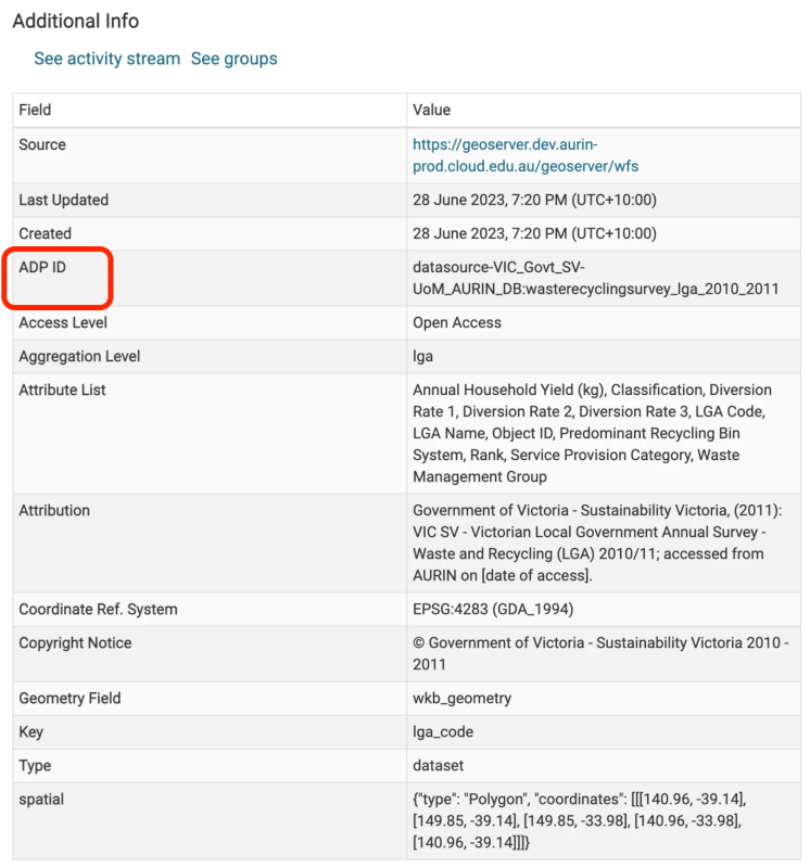
To download that dataset into R, find and copy its ADP ID in the metadata table. In this case the ADP ID is datasource-VIC_Govt_SV-UoM_AURIN_DB:wasterecyclingsurvey_lga_2010_2011. Then create the following query, pasting the ADP ID into the typeName variable within RStudio.

req <- request(wfs_url) %>%
   req_url_query(
     "request" = "GetFeature",
     "typeName" = "datasource-VIC_Govt_SV-UoM_AURIN_DB:wasterecyclingsurvey_lga_2010_2011",
     "srsName" = "EPSG:4326"
) %>% 
req_auth_basic(user_name, password)

Use the following functions to build the query and download the data from the API and save it. In this case we are downloading the data in GML format and saving it with the file name data_recycling.gml. You can see a list of other supported output formats here.

resp <- req |> req_perform() |> resp_body_string()
### ---- Write the data to a file ---- ###
write(resp,"data_recycling.gml")
### ---- Read the data ---- ####
data <- read_sf("data_recycling.gml")

d) View data

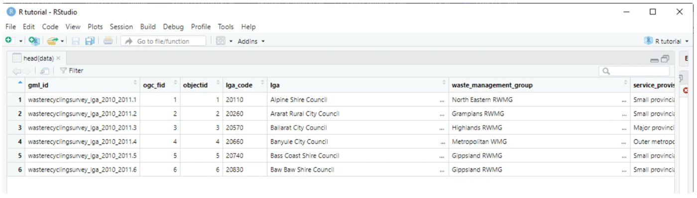
Use the head() function again to view some of the dataset’s rows:

head(data)

The output should consist of information about the waste and recycling services in tabular format:

e) Visualise data

Use the mapview() function to visualise the dataset:

mapview(data)

You should now see the Local Government Areas (LGAs) in Victoria represented on a map in the ‘Viewer’ tab.

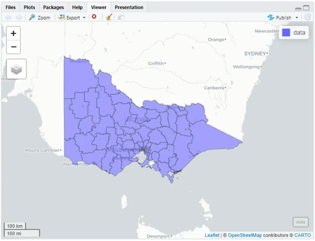
Clicking an LGA on the map will reveal information about the waste & recycling service in that LGA.

f) Filter data by bounding box

The API supports spatial queries that permit filtering your data in a particular spatial area. For example, you can filter the data by bounding box (BBOX). By adding the BBOX, instead of downloading entire datasets, which can be very large and irrelevant to your project, you can download data according to your specific geographic area of interest. Here we show an example to use the Melbourne CBD as the area of interest.

The BBOX parameter allows you to search for features that are contained (or partially contained) inside a box of user-defined coordinates. The format of the BBOX parameter is bbox=a1,b1,a2,b2,[crs] where a1, b1, a2, and b2 represent the coordinate values.

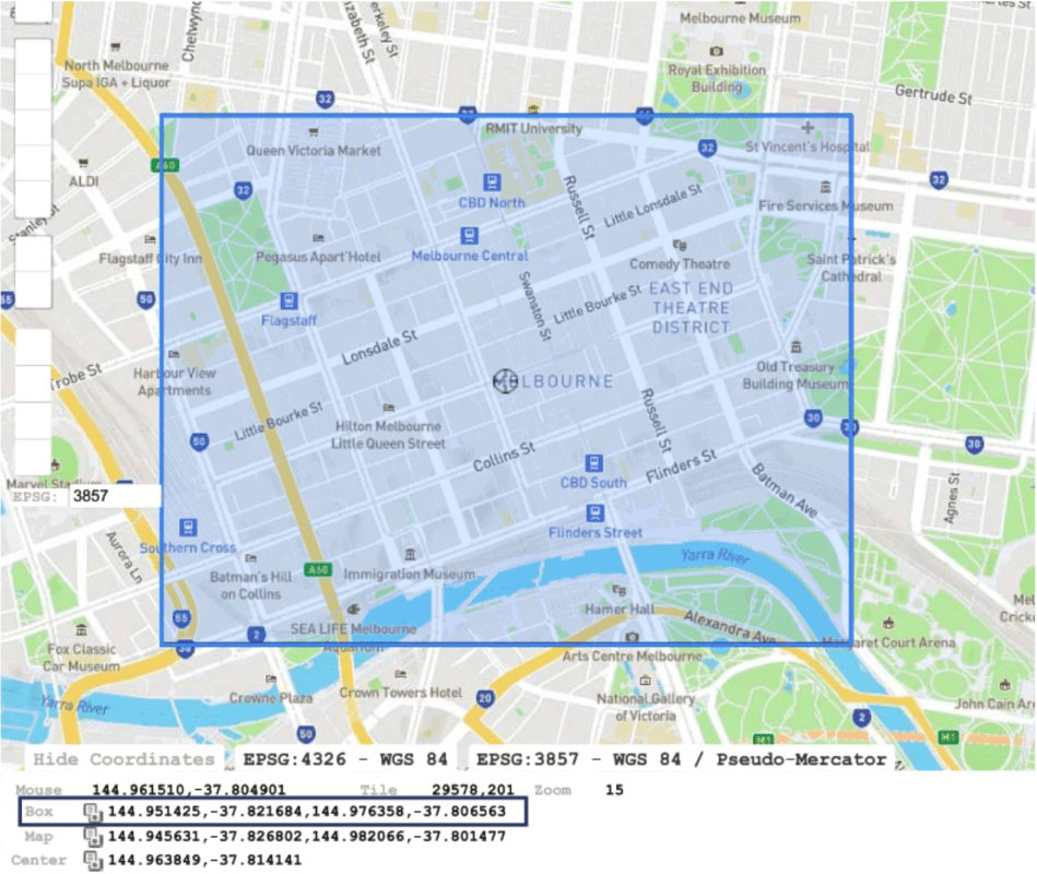
We recommend using BBox finder to create your BBOX using a base map. Click the rectangle icon and draw a rectangle using your mouse to cover the Melbourne CBD area or any other areas you are interested in.

Now you can see the selected rectangle is covered in pink. You may check if it is the right area from which you wish to collect data. Copy the BBOX coordinates from the highlighted area and replace the coordinates after the code bbox =.

You also need to replace “yourName” and “yourPassword” in the code block below with your API username and password, which again can be found under ‘Manage Access’ → ‘API Access’ after you’ve logged in. If you don’t have API credentials, please generate your credentials via the Access Dashboard.

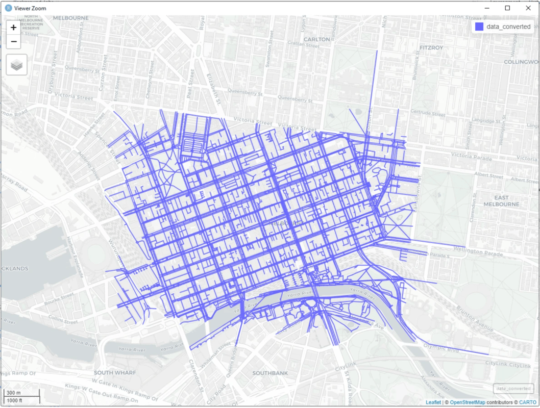
Finally, you will need to copy and paste the ‘ADP_ID’ from the metadata in the data catalogue for your chosen dataset. For this example, we will be using the ‘OpenStreetMap – Roads and Paths – Lines (Australia) 2021’ dataset. We will be converting the dataset’s geometry type from “MULTICURVE” to “MULTILINESTRING” in order to allow the “mapview” package to display it properly.

###### ------ Libraries ------- ####
library(sf)
library(httr2)
library(ows4R)
library(mapview)
library(utils)

##### ----- Credentials ------ #####
wfs_url <- "https://adp.aurin.org.au/geoserver/wfs"
user_name <- "yourName"
password <- "yourPassword"

#### ------ Select the data set ----- #####
ADP_ID = 'datasource-OSM-UoM_AURIN_DB:osm_roads_2021'

### ------ Copy vector from http://bboxfinder.com/ ---- #####
bbox = '144.951425,-37.821684,144.976358,-37.806563'

### ------ Copy vector from http://bboxfinder.com/ ---- #####
bbox = '144.927135,-37.828836,145.000648,-37.799408'

### ------ Create request ---- #####
req <- request(wfs_url) %>%
    req_url_query(
        service = "WFS",
        version = "2.0.0",
        request = "GetFeature",
        typeName = ADP_ID,
        bbox=paste0(bbox,',EPSG:4326'),
        srsName = "EPSG:4326"
     )%>%
    req_auth_basic(user_name, password)
resp <- req |> req_perform() |> resp_body_string()

#### ---- Write the data to a file ----- ####
write(resp,"data_bbox.gml")
### ---- Read the data ---- ####
data <- read_sf("data_bbox.gml")
### ---- Choose a specific geometry type (e.g., "MULTILINESTRING") ---- ###
selected_geometry_type <- "MULTILINESTRING"
### ---- Convert the data's geometry type to "MULTILINESTRING" ---- ###
data_converted <- st_cast(data, to = selected_geometry_type)
### --- Show the map with the converted data --- ###
mapview(data_converted)

Output: