LEARN TO explore
Accessing the AURIN API via PYTHON
This tutorial is also available on the following GitHub repository:  GitHub – AURIN-OFFICE/training
This tutorial introduces how to use Python to connect to the AURIN API or to access and download the AURIN data. This is designed with no prerequisite of Python experience.
The AURIN Application Programming Interface (API), is an interface that allows you to use a programming language to interact with an application, and perform tasks such as getting data, updating data, or deleting data. The AURIN API is such an interface that allows users to access data and metadata available from the AURIN Data Catalogue. You can send a request to the API using Python scripts and get a response to download specific datasets. The API is based on Open Geospatial Consortium Web Feature Service (WFS) Interface Standards.
Before commencing this step, please ensure you have generated your unique API Access Credentials (username and password) using the AURIN Access Dashboard. If you need guidance on creating your credentials, please refer to the tutorial here.
Please note the API access password will expire in 90 days for security reasons. You can always get a new password by visiting the API Access page.
Tutorial Goals
In this tutorial, our goal is to use a Python script to connect to the ADP and download a dataset. You will learn how to:
-
Choose between different Python environments
-
Install related Python packages
-
Use Python coding environments
-
Interact with the AURIN API
a. Setup connection parameter
b. List available datasets
c. Download data
d. View data
e. Visualise data
f. Download data in other formats
g. Filter data by bounding box
1. Choose Between Different Python Environments
Python is a free and open-source high-level, interpreted, general-purpose programming language. It is widely used in data science and has become a very powerful tool for data analysts from all disciplines, from economics to ecology and geography. The geographic information system (GIS) capabilities of Python have developed significantly over the last decade.
If you are getting started with Python, we suggest you use a cloud environment, such as Google Colab, as it has Python and some libraries already installed. If you wish to use your personal computer, we recommend using Python version 3.7.0 or later. We hope the image below may help you understand the benefits and limitations of each option.

a. Cloud Environment: Google Colab
Google Colab has an option of free Google research environment for users with a Google account. Google Colab has tutorials and blogs for you to learn the basics about this cloud environment. Here are the links: Google Colaboratory
 Google Colab – Medium
Open a new Python notebook: click File → New notebook. Please sign in with your Google account.
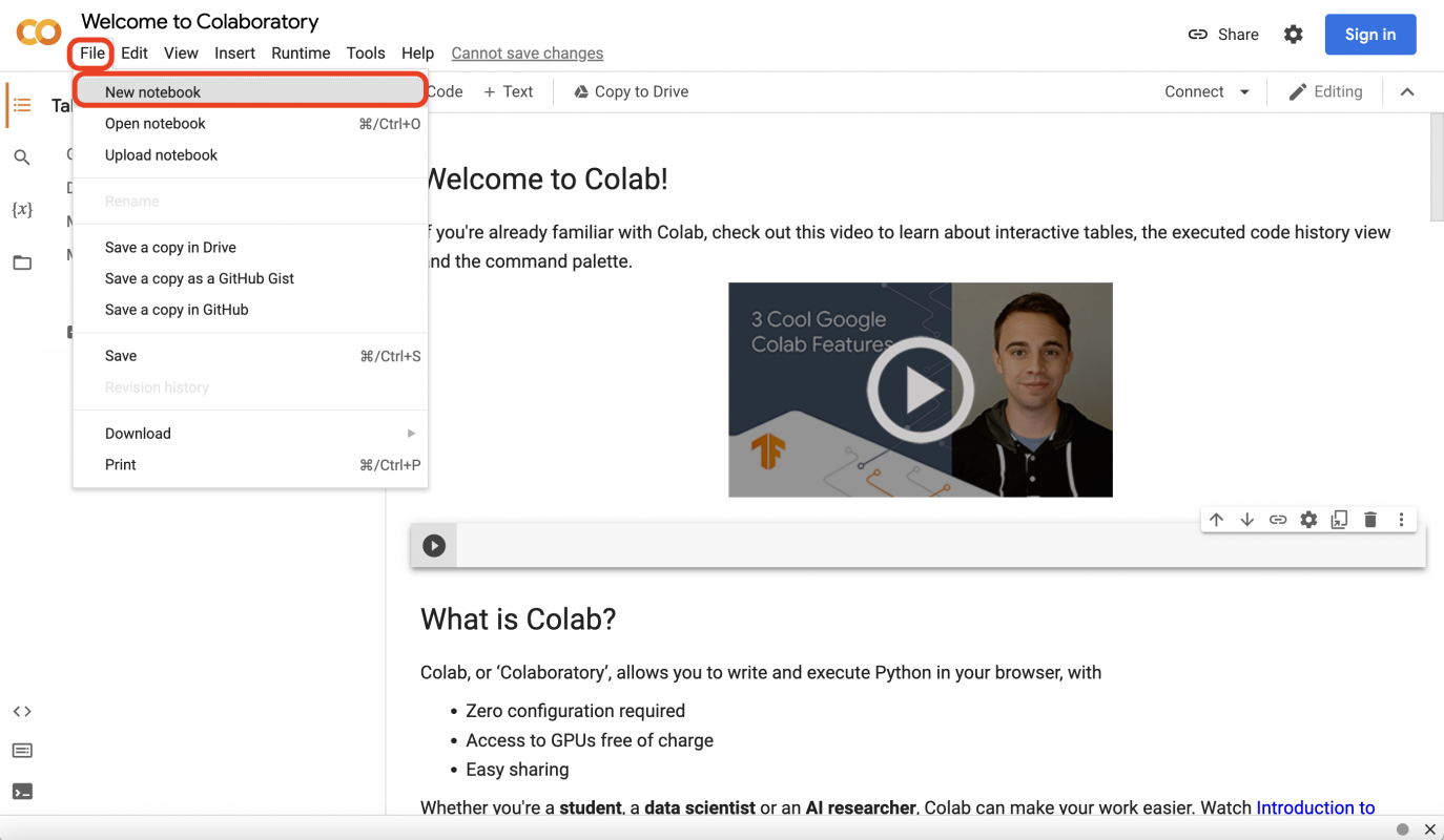
This will bring you to a new notebook environment and you are ready for the first line of code.

b. Local Environment
You can download Python from Python.org.
If you’d like to install JupyterLab, please visit ![]() Installation — JupyterLab 4.1.4 documentation. We recommend Jupyter Notebook, or JupyterLab on your local machine, instead of a vanilla py file, to be able to see the graphs and maps presented below.
Installation — JupyterLab 4.1.4 documentation. We recommend Jupyter Notebook, or JupyterLab on your local machine, instead of a vanilla py file, to be able to see the graphs and maps presented below.
2. Python packages and Libraries
Python packages are libraries of Python functions developed by the Python community. We can import these packages to our Python scripts to add functionality. For this tutorial, we need to use the following Python packages:
-
OWSLib (version 0.29.3)
-
Fiona (version 1.9.5)
-
GeoPandas (version 0.12.2)
-
folium (version 0.13.0)
-
requests (version 2.31.0)
The versions specified here are recommendations. This may be different depending on your python environment. Please feel free to adjust versions to fit your python environment.
OWSLib is a Python package that we use to connect to the API.
Fiona and GeoPandas are libraries to make working with geospatial data.
Folium makes it easy to visualise data.
Requests is a simple, yet elegant, HTTP library. It is a HTTP library used for making requests to web servers, abstracting the complexities of making requests behind a simple API.
3. Use Python coding environments
Now is the time to introduce how to use the Python coding environment. We use Google Colab as an example. Open a new notebook in Colab.
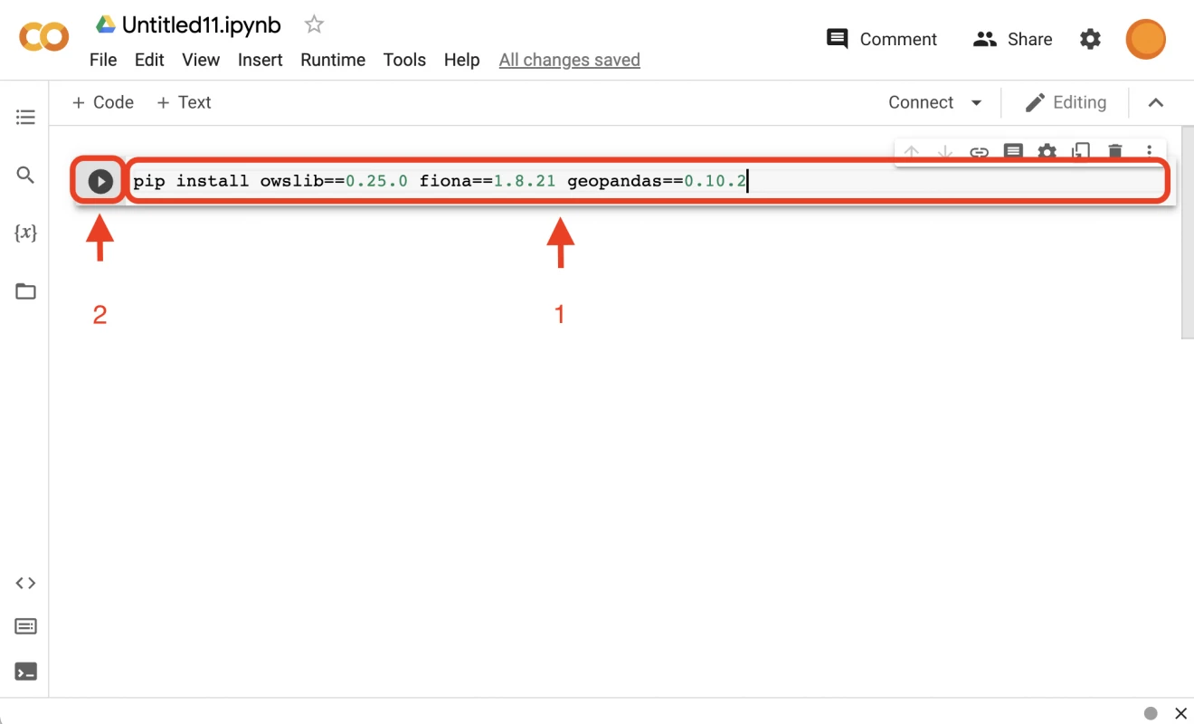
You can install all of the related Python packages in Section 2 using the following command. The pip install <package> command always looks for the latest version of the package and installs it. If we’d like to install a specific version, we can use ==, then follow the version number, for example, owslib==0.29.3. (The library versions specified below are tested for Google Colab environment. For local environment, these versions may vary.)
pip install owslib==0.29.3 fiona==1.9.5 geopandas==0.14.1 requests==2.31.0 folium==0.15.1
Add a Code cell
Step 1, you can copy and paste the install command above into the Code cell.
Step 2, execute the command by clicking the run button.
We recommend this short video to learn more about the Jupyter notebook environment ![]() Get started with Google Colaboratory (Coding TensorFlow)
Get started with Google Colaboratory (Coding TensorFlow)
After the installation of Python packages, we can load these packages for coding later. To load these packages, we use command import. WebFeatureService is the function we use in OWSLib. If you’d like to know the meanings of library, module, function, import, etc. please click here.
Load the packages and additional functions:
from owslib.wfs import WebFeatureService
import geopandas
import folium
import io
Add another line of code
Click +Code button, and then a new code cell is added to the environment. You can then copy and paste the import command above and execute it.

Add a text cell
Click +Text button, and then a text cell is added to the environment. In a text cell, you may like to add some textual explanation of the code. You need to use the Markdown format for text editing.
Please find out more in this Markdown Guide. The left hand side is the textual input and the right hand side displays the final appearance in the notebook.
When you finish editing and move to the next cell, it will automatically jump out of the editing mode, and appear on the right-hand side.

4. Interact with the AURIN API
a. Setup Connection Parameters
To use an API, you make a request to AURIN’s remote web server and retrieve the data you need.
To connect to the API you need to let Python know the address for the request and your credentials.
Please replace yourName and yourPassword in the code block below with your API Access username and password. If you don’t have credentials, please generate your credentials via API Access Dashboard or if you need guidance on creating your credentials, please refer to the tutorial here.
Please note the API access password will expire in 90 days for security reasons. You can always get a new password by visiting the API Access page.
WFS_USERNAME = 'yourName'
WFS_PASSWORD= 'yourPassword'
WFS_URL='https://adp.aurin.org.au/geoserver/wfs'
Create a new api_client, using the below code to connect to the ADP, which is itself a Web Feature Service (WFS).
api_client = WebFeatureService(url=WFS_URL,username=WFS_USERNAME, password=WFS_PASSWORD, version='1.1.0')b. List Available Datasets
We can view the WFS operations.
# (Optional) Check what operations are available
[operation.name for operation in api_client.operations]
Output:
['GetCapabilities',
'DescribeFeatureType',
'GetFeature',
'GetGmlObject',
'LockFeature',
'GetFeatureWithLock',
'Transaction']
We can view information about the dataset name and title of the first 10 datasets:
# (Optional) Check what datasets are available
contents = list(api_client.contents)
contents[:10]
Output:
['datasource-NSW_Govt_DPE-UoM_AURIN_DB:nsw_srlup_additional_rural_2014',
'datasource-AU_Govt_ABS-UoM_AURIN_DB_GeoLevel:aus_2016_aust',
'datasource-AU_Govt_ABS-UoM_AURIN_DB_GeoLevel:gccsa_2011_aust',
'datasource-AU_Govt_ABS-UoM_AURIN_DB_GeoLevel:gccsa_2016_aust',
'datasource-AU_Govt_ABS-UoM_AURIN_DB_GeoLevel:mb_2016_aust',
'datasource-AU_Govt_ABS-UoM_AURIN_DB_GeoLevel:mb_2011_act',
'datasource-AU_Govt_ABS-UoM_AURIN_DB_GeoLevel:mb_2011_nsw',
'datasource-AU_Govt_ABS-UoM_AURIN_DB_GeoLevel:mb_2011_nt',
'datasource-AU_Govt_ABS-UoM_AURIN_DB_GeoLevel:mb_2011_ot',
'datasource-AU_Govt_ABS-UoM_AURIN_DB_GeoLevel:mb_2011_qld']
c. Download Data
You can search the AURIN Data Catalogue to find datasets you would like to download.
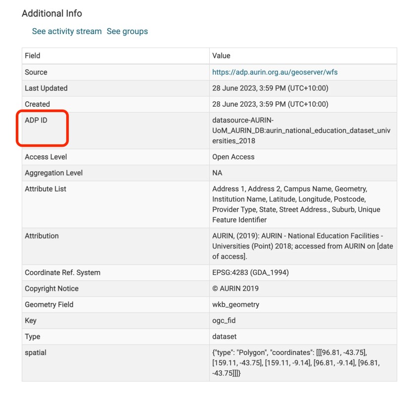
For example, if you are interested in a dataset describing the university institutes in Australia, enter “university” and click search. Browse the results and select AURIN – National Education Facilities – Universities (Point) 2018 and view its description, including its metadata table.
To download that dataset into Python, find and copy its ADP ID Value from the metadata table, in this case, it is datasource-AURIN-UoM_AURIN_DB:aurin_national_education_dataset_universities_2018.
Then create the following query, pasting the ADP ID into the type name variable. The GetFeature() operation returns a selection of features from the data source. Then we save it to the variable called response.
response = api_client.getfeature(typename='datasource-AURIN-UoM_AURIN_DB:aurin_national_education_dataset_universities_2018')Next, save the variable response to a file named data_uni.gml. This file is in gml format, and ‘gml’ is the default WFS output format. If you’d like to download the dataset, please store it in a safe and secure environment.
out = open('data_uni.gml', 'wb')out.write(response.read())out.close()
d. View Data
After downloading the information, we can use the function geopandas.read_file to load the data in a DataFrame.
Use the head() function to see universities on a map as individual point locations:
data_uni = geopandas.read_file('data_uni.gml')data_uni.head()Now you will see information about the universities in tabular format:

e. Visualise Data
Static Map
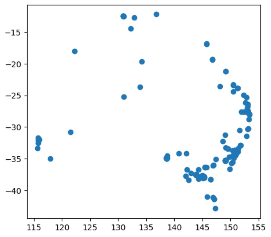
You can now visualise the universities on a map as individual point locations by using the plot() command. If you are using Mac, you may need to install matplotlib manually to get the visualisation from the plot() function. (Here are two references for matplotlib installation on Mac: Installation — Matplotlib 3.8.3 documentation and
![]() How to Install Matplotlib on MacOS? – GeeksforGeeks. Please remember to
How to Install Matplotlib on MacOS? – GeeksforGeeks. Please remember to import matplotlib after installation).
data_uni.plot()
Output:
Interactive Map
Here we set up an interactive map to view the Australian universities dataset. The function folium.map creates an interactive map.
### ----- Define the basemap: Center: Australia ---- ###
Map_aurin = folium.Map(location=[-23.43046024417681, 133.6034805654919],zoom_start=4,tiles='cartodbpositron')
### ----- Select Name and Geometry ---- ###
map_data = data_uni[['institution','geometry']]
### ----- Create a JSON with the information ------ ###
layer = map_data.to_json()
### --- Geojson -- ###
folium.GeoJson(layer,name='geojson').add_to(Map_aurin)
# Show the map again
Map_aurin
Output:

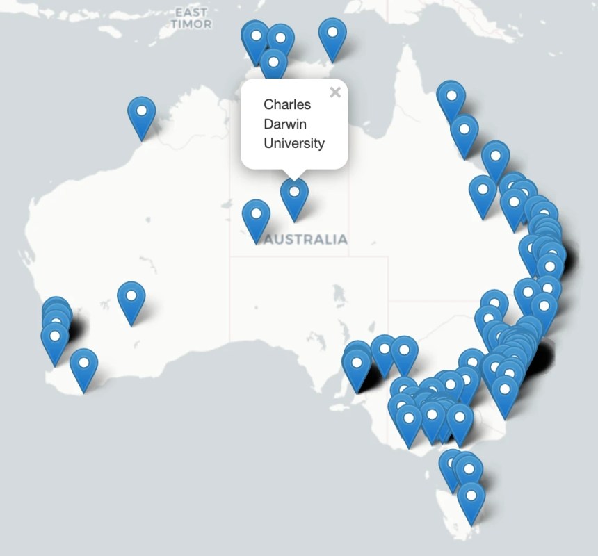
You may wish to click on the tag and see which institute it is. Here is the code added the popup function with institution’s names.
# Make an empty map
Map_aurin = folium.Map(location=[-23.43046024417681, 133.6034805654919],zoom_start=4,tiles='cartodbpositron')

# add marker one by one on the map
for i in range(0,len(data_uni)):
    folium.Marker(
      location=[data_uni.iloc[i]['latitude'],data_uni.iloc[i]['longitude']],
      popup=data_uni.iloc[i]['institution'],
    ).add_to(Map_aurin)

# Show the map again
Map_aurin
Output:
f. Download Data in other Formats
The AURIN API supports other data formats, such as GeoJSON, CSV, GML, KML, etc. For a full list of different formats and their syntax for coding, please check here. We choose the GeoJSON format for demonstration.
GeoJSON format, download data and visualisation. outputFormat='application/json' helps to specify GeoJSON format.
response = api_client.getfeature(typename='datasource-AURIN-UoM_AURIN_DB:aurin_national_education_dataset_universities_2018',outputFormat='application/json')
out = open('data_uni.geojson', 'wb')
out.write(response.read())
out.close()
data_uni = geopandas.read_file('data_uni.geojson')
g. Filter Data by Bounding Box
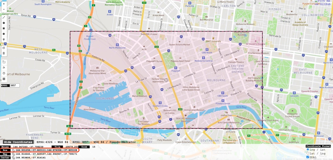
The AURIN API supports spatial queries that permit filtering your data in a particular spatial area. For example, you can filter the data by bounding box (BBOX). By adding the BBOX, instead of downloading entire datasets, which can be very large and irrelevant to your project, you can download data according to your area of interest. Here we show an example to use the Melbourne CBD as the area of interest. The BBOX is a function from shapely.geometry.
The BBOX parameter allows you to search for features that are contained (or partially contained) inside a box of user-defined coordinates. The format of the BBOX parameter is bbox=a1,b1,a2,b2,[crs] where a1, b1, a2, and b2 represent the coordinate values, crs refers to the coordinate reference system. If you’d like to know more about Australian geospatial reference system, please click here. The shapely.geometry.box() function makes a rectangular polygon from the provided BBOX parameters.
We recommend using BBox finder to create your BBOX using a base map. Click the rectangle icon and draw a rectangle using your mouse to cover the Melbourne CBD area or any other areas you are interested in.

Now you can see the selected rectangle is covered in pink. You may check if it is the right area you’d like to collect data from. Copy the BBOX coordinates from the highlighted area, and replace the coordinates after the code min_x,min_y,max_x,max_y =.
You also need to replace yourName and yourPassword in the code block below with your API Access username and password. If you don’t have API credentials, please generate your credentials via the AURIN Access Dashboard.
###### ------ Libraries ------- ####
from owslib.wfs import WebFeatureService
import geopandas as gpd
from shapely.geometry import box
import io
import folium

##### ----- Credentials ------ #####
WFS_USERNAME = 'yourName'
WFS_PASSWORD= 'yourPassword'
VERSION = '1.1.0'
WFS_URL='https://adp.aurin.org.au/geoserver/wfs'
api_client = WebFeatureService(url=WFS_URL,
    username=WFS_USERNAME,
    password=WFS_PASSWORD,
    version=VERSION)

#### ------ Select the data set ----- #####
ADP_ID = 'datasource-AURIN-UoM_AURIN_DB:aurin_national_education_dataset_universities_2018'

### ------ Copy vector from http://bboxfinder.com/ ---- #####
min_x,min_y,max_x,max_y = 144.931258,-37.823111,144.976358,-37.805108

# Create the polygon using Shapely
box_shape = box(minx=min_x, miny=min_y, maxx=max_x, maxy=max_y)
Box_shape = gpd.GeoDataFrame({'box': 'Box','geometry': [box_shape]})

#### ------ Request data for Melbourne CBD ----- ####
response = api_client.getfeature(typename = ADP_ID,bbox=(min_x, min_y, max_x, max_y), srsname='urn:ogc:def:crs:EPSG::4326')

#### ---- Storage data ----- ####
with open('data_uni.gml', 'wb') as f:
   f.write(response.read())
data_uni = gpd.read_file('data_uni.gml')

### ----- Define the basemap: Center: Australia ---- ###
Map_aurin = folium.Map(location=[box_shape.centroid.coords[0][1],box_shape.centroid.coords[0][0]],zoom_start=15,tiles='cartodbpositron')

### ----- Select Name and Geometry ---- ###
### ----- Create a JSON with the information ------ ###
map_data = data_uni[['institution','geometry']]
### ---- Features box ----- ###
layer = map_data.to_json()
### ---- Shape box ---- ###
box = Box_shape.to_json()
### --- Geojson -- ###
folium.GeoJson(layer,name='features').add_to(Map_aurin)
folium.GeoJson(box,name='box',style_function = lambda x: {'fillColor': 'yellow'}).add_to(Map_aurin)

# add marker one by one on the map
for i in range(0,len(data_uni)):
   folium.Marker(
     location=[data_uni.iloc[i]['latitude'],data_uni.iloc[i]['longitude']],
     popup=data_uni.iloc[i]['institution'],
   ).add_to(Map_aurin)

### --- Show the map --- ###
Map_aurin
Output:


